AlexNet 논문 리뷰 및 해석
22 Apr 2020ImageNet Classification with Deep Convolutional Neural Networks
Abstract
We trained a large, Deep convolutional neural network to classify the 1.2 million high-resolution images in the ImageNet LSVRC-2010 contest into the 1000 different classes.
ImagesNet LSVRC-2010 대회에서 120만 고해상도 이미지를 1000가지 클래스로 분류하기 위해 대규모 Deep convolutioal neural network을 훈련했습니다.
On the test data, we achieved top-1 and top-5 error reates of 37.5% and 17.0% which is considerably better than the previous state-of-the-art.
테스트 데이터에서 우리는 37.5% 및 17.0%의 상위-1 및 상위-5 오류율을 달성했으며 이는 이전의 최신 기술보다 훨씬 우수합니다.
The neural network, which has 60 million parameters and 650,000 neurons, consists of five convolutional layers, some of which are followed by max-pooling layers, and threefully-connected layers with a final 1000-way softmax.
6천만개의 매개 변수와 650,000개의 뉴런을 갖는 신경망은 5개의 컨볼루션 레이어로 구성되며, 그 중 일부는 max-pooling 레이어와 3개의 완전히 연결된 레이어와 최종 1000-way softmax로 구성됩니다.
To make training faster, we used non-saturating neurons and a very efficient GPU implementation of the convolution operation.
훈련 속도를 높이기 위해
비 포화 뉴런과 컨볼루션 연산의 매우 효율적인 GPU 구현을 사용했습니다.
To reduce overfitting in the fully-connected layers we employed a recently-developed regularization method called “dropout” that proved to be very effective.
완전히 연결된 레이어에서
과적합을 줄이기 위해 최근에 개발 된 “드롭 아웃”이라는 정규화 방법을 사용하였으며 매우 효과적이었습니다.
We also entered a variant of this model in the ILSVRC-2012 competition and achieved a winning top-5 test error rate of 15.3%, compared to 26.2% achieved by the second-best entry.
또한 ILSVRC-2012 경쟁에서 이 모델의 변형을 도입하여 2위를 차지한 26.2%와 비교하여 15.3%의 상위 5개 테스트 오류율을 달성했습니다.
1. Introduction
Current approaches to object recognition make essential use of machine learning methods.
객체 인식에 대한 현재 접근 방식은 기계 학습 방법을 필수적으로 사용합니다.
To improve their performance, we can collect larger datasets, learn more powerful models, and use better techniques for preventing overfitting.
성능을 향상시키기 위해 더 큰 데이터 세트를 수집하고 더 강력한 모델을 배우며 오버 피팅을 방지하기 위해 더 나은 기술을 사용할 수 있습니다.
Until recently, datasets of labeled images were relatively small — on the order of tens of thousands of images (e.g., NORB [16], Caltech-101/256 [8, 9], and CIFAR-10/100 [12]).
최근까지 라벨이 있는 이미지의 데이터 세트만 수 만개의 이미지(예 NORB[16], Caltech-101/256[8,9], and CIFAR-10/100[12])정도로 상대적으로 작았습니다.
Simple recognition tasks can be solved quite well with datasets of this size, especially if they are augmented with label-preserving transformations.
특히 라벨 보존 변형으로 보강된 경우, 이 크기의 데이터 세트를 사용하면 간단한 인식 작업을 매우 잘 해결할 수 있습니다.
For example, the currentbest error rate on the MNIST digit-recognition task (<0.3%) approaches human performance [4].
예를 들어, MNIST 숫자 인식 작업에서 현재 최고 오류율(<0.3%)은 인간의 성과에 근접합니다.
But objects in realistic settings exhibit considerable variability, so to learn to recognize them it is necessary to use much larger training sets. And indeed, the shortcomings of small image datasets have been widely recognized (e.g., Pinto et al. [21]), but it has only recently become possible to collect labeled datasets with millions of images.
그러나 사실적인 설정의 객체는 상당한 변동성을 나타내므로 이를 인식하려면 훨씬 더 큰 훈련 세트를 사용 해야 합니다. 실제로 작은 이미지 데이터 세트의 단점이 널리 인식되고 있지만(예 : Pinto et al[21])최근에는 수 백만 개의 이미지로 레이블이 지정된 데이터 세트를 수집하는 것이 가능해졌습니다.
The new larger datasets include LabelMe [23], which consists of hundreds of thousands of fully-segmented images, and ImageNet [6], which consists of over 15 million labeled high-resolution images in over 22,000 categories.
더 큰 새로운 데이터 세트에서 수십만 개의 완전 분할 된 이미지로 구성된 LabelMe[23] 및 22,000개 이상의 카테고리에서 1,500만개 이상의 레이블이 있는 고해상도 이미지로 구성된 ImageNet[6]이 포함됩니다.
To learn about thousands of objects from millions of images, we need a model with a large learning capacity.
수 백만개 이미지에서 수 천개의 물체에 대해 배우려면 큰 학습 능력을 갖춘 모델이 필요합니다.
However, the immense complexity of the object recognition task means that this problem cannot be specified even by a dataset as large as ImageNet, so our model should also have lots of prior knowledge to compensate for all the data we don’t have.
그러나 객체 인식 작업의 복잡성으로 인해 ImageNet만큼 큰 데이터 집합으로도 이 문제를 지정할 수 없으므로 모델에 없는 모든 데이터를 보완 할 수 있는 사전 지식이 많이 있어야 합니다.
Convolutional neural networks (CNNs) constitute one such class of models [16, 11, 13, 18, 15, 22, 26].
CNN(Convolutional Neural Networks)은 그러한 종류의 모델을 구성합니다[16, 11, 13, 18, 15, 22, 26].
Their capacity can be controlled by varying their depth and breadth, and they also make strong and mostly correct assumptions about the nature of images (namely, stationarity of statistics and locality of pixel dependencies).
깊이와 폭을 변경하여 용량을 제어 할 수 있으며, 이미지의 특성(즉, 통계의 정상성 및 픽셀 종속성의 국소성)에 대해 강력하고 대부분 정확한 가정을 합니다.
Despite the attractive qualities of CNNs, and despite the relative efficiency of their local architecture, they have still been prohibitively expensive to apply in large scale to high-resolution images.
CNN의 매력적인 특정과 로컬 아키텍처의 상대적 효율성에도 불구하고, 그들은 고해상도 이미지에 대규모로 적용하기에는 여전히 엄청난 비용이 들었습니다.
Luckily, current GPUs, paired with a highly-optimized implementation of 2D convolution, are powerful enough to facilitate the training of interestingly-large CNNs, and recent datasets such as ImageNet contain enough labeled examples to train such models without severe overfitting.
다행히도, 현재의 GPU는 2D 컨볼루션의 최적화된 구현과 함께 규모가 큰 CNN의 훈련을 용이하게 할 만큼 강력하며, ImageNet과 같은 최근의 데이터 세트는 심한 과적합 없이 모델을 교육하기에 충분한 레이블이 있는 예제가 포함되어 있습니다.
The specific contributions of this paper are as follows: we trained one of the largest convolutional neural networks to date on the subsets of ImageNet used in the ILSVRC-2010 and ILSVRC-2012 competitions [2] and achieved by far the best results ever reported on these datasets.
이 논문의 구체적인 기여는 다음과 같습니다. 우리는 ILSVRC-2010 및 ILSVRC-2012 대회에 사용 된 ImageNet의 하위 집합[2]에 대해 현재까지 가장 큰 컨볼루션 신경망 중 하나를 교육했으며, 이러한 데이터 세트에 대해 지금까지 보고 된 최고의 결과를 달성했습니다.
We wrote a highly-optimized GPU implementation of 2D convolution and all the other operations inherent in training convolutional neural networks, which we make available publicly.
우리는 2D 컨볼루션 신경망 훈련에 내재 된 다른 모든 작업에 대해 최적화 된 GPU 구현을 작성하여 공개적으로 사용할 수 있게 했습니다.[http://code.google.com/p/cuda-convnet/]
Our network contains a number of new and unusual features which improve its performance and reduce its training time, which are detailed in Section 3.
우리의 네트워크는 성능을 향상시키고 훈련 시간을 단축시키는 여러 가지 새롭고 특이한 특징들을 포함하고 있는데, 이는 섹션 3에 자세히 설명되어 있습니다.
The size of our network made overfitting a significant problem, even with 1.2 million labeled training examples, so we used several effective techniques for preventing overfitting, which are described in Section 4.
네트워크 규모가 120만 개에 달하는 훈련 된 예에서도 과도하게 큰 문제를 야기 시켰으며, 우리는
오버피팅을 방지하기 위해 몇 가지 효과적인 기술을 사용했으며, 이는 섹션 4에 설명되어 있습니다.
Our final network contains five convolutional and three fully-connected layers, and this depth seems to be important: we found that removing any convolutional layer (each of which contains no more than 1% of the model’s parameters) resulted in inferior performance.
우리의 최종 네트워크는 5개의 컨볼루션 레이어와 3개의 완전 연결 레이어를 포함하고 있으며, 이 깊이는 중요한 것으로 보입니다: 우리는 어떤 컨볼루션 레이어(각각 모델 매개변수의 1% 이하 포함)를 제거하면 성능이 저하된다는 것을 발견했습니다.
In the end, the network’s size is limited mainly by the amount of memory available on current GPUs and by the amount of training time that we are willing to tolerate.
결국, 네트워크의 크기는 주로 현재 GPU에서 사용할 수 있는 메모리 양과 허용할 수 훈련 시간에 의해 제한됩니다.
Our network takes between five and six days to train on two GTX 580 3GB GPUs.
우리의 네트워크는 2개의 GTX 580 3GB GPU를 훈련시키는 데 5일에서 6일이 걸립니다.
All of our experiments suggest that our results can be improved simply by waiting for faster GPUs and bigger datasets to become available.
모든 실험에서 더 빠른 GPU와 더 큰 데이터 세트를 사용할 수 있을 때까지 기다리면 결과를 개선할 수 있다고 제안합니다.
2. The Dataset
ImageNet is a dataset of over 15 million labeled high-resolution images belonging to roughly 22,000 categories.
ImageNet은 약 22,000개 범주에 속하는 1,500만개 이상의 고해상도 이미지의 데이터 세트입니다.
The images were collected from the web and labeled by human labelers using Amazon’s Mechanical Turk crowd-sourcing tool.
웹에서 이미지를 수집하고 Amazon Mechanical Turk 크라우드 소싱 도구를 사용하여 인간 라벨러들이 라벨을 지정했습니다.
Starting in 2010, as part of the Pascal Visual Object Challenge, an annual competition called the ImageNet Large-Scale Visual Recognition Challenge (ILSVRC) has been held.
2010년부터 Pascal Visual Object Challenge의 일환으로 매년 ImageNet Large-Scale Visual Recognition Challenge (ILSVRC)라는 대회가 개최되었습니다.
ILSVRC uses a subset of ImageNet with roughly 1000 images in each of 1000 categories. In all, there are roughly 1.2 million training images, 50,000 validation images, and 150,000 testing images.
ILSVRC는 1000개 범주 각각에 약 1000개의 이미지가 있는 ImageNet의 하위 세트를 사용합니다. 총 120만 개의 교육이미지, 50,000개의 유효성 검사 이미지 및 150,000개의 테스트 이미지가 있습니다.
ILSVRC-2010 is the only version of ILSVRC for which the test set labels are available, so this is the version on which we performed most of our experiments.
ILSVRC-2010은 테스트 세트의 레이블을 사용할 수 있는 유일한 ILSVRC 버전이므로 대부분의 실험을 수행 한 버전입니다.
Since we also entered our model in the ILSVRC-2012 competition, in Section 6 we report our results on this version of the dataset as well, for which test set labels are unavailable.
우리는 ILSVRC-2012 경쟁에서도 우리의 모델을 입력하였기 때문에, 섹션6에서는 테스트 세트 라벨을 사용할 수 없는 이 버전의 데이터 집합에 대한 우리의 결과도 보고합니다.
On ImageNet, it is customary to report two error rates: top-1 and top-5, where the top-5 error rate is the fraction of test images for which the correct label is not among the five labels considered most probable by the model.
ImageNet에서 상위 1 및 상위 5의 두 가지 오류율을 보고하는 것이 일반적입니다. 여기서 상위 5 오류율은 올바른 레이블이 모델에서 가장 가능성이 높은 것으로 간주되는 5개의 레이블 중 하나가 아닌 테스트 이미지의 일부입니다.
ImageNet consists of variable-resolution images, while our system requires a constant input dimensionality.
ImageNet은 가변 해상도 이미지로 구성되며, 시스템에는 일정한 입력 크기가 필요합니다.
Therefore, we down-sampled the images to a fixed resolution of 256 × 256. Given a rectangular image, we first rescaled the image such that the shorter side was of length 256, and then cropped out the central 256×256 patch from the resulting image.
따라서 이미지를 고정 해상도 256 * 256 으로 다운 샘플링했습니다. 직사각형 이미지를 고려할 때 먼저 짧은 면의 길이가 256이 되도록 이미지의 크기를 조정한 다음 결과에서 중앙 256 * 256 패치를 자릅니다.
We did not pre-process the images in any other way, except for subtracting the mean activity over the training set from each pixel.
각 픽셀에서 훈련 세트에 대한
평균 활동을 빼는 것을 제외하고는 다른 방법으로 이미지를 사전 처리하지 않았습니다.
So we trained our network on the (centered) raw RGB values of the pixels.
그래서 우리는
픽셀의 (중심) 처음 RGB 값에 대해 네트워크를 학습했습니다.
3. The Architecture
The architecture of our network is summarized in Figure 2.
네트워크의 아키텍처는 그림2 에 요약되어 있습니다.
It contains eight learned layers — five convolutional and three fully-connected.
여기에는 8개의 학습 레이어(5개의 회선 및 3개의 완전히 연결된 레이어)가 포함됩니다.
Below, we describe some of the novel or unusual features of our network’s architecture.
아래에서는 네트워크 아키텍쳐의 새롭거나 특이한 기능에 대해 설명합니다.
Sections 3.1-3.4 are sorted according to our estimation of their importance, with the most important first.
섹션 3.1 - 3.4는 중요성에 대한 우리의 추정에 따라 가장 중요한 것부터 정렬됩니다.
3.1 ReLU Nonlinearity
The standard way to model a neuron’s output f as a function of its input $x$ is with $f(x) = tanh(x)$ or $f(x) = (1 + e ^{−x})^{−1}$.
입력 $x$의 함수로 뉴런의 출력 f를 모델링하는 표준 방법은 $f(x) = tanh(x)$ 또는 $f(x) = (1 + e ^{−x})^{−1}$입니다.
In terms of training time with gradient descent, these saturating nonlinearities are much slower than the non-saturating nonlinearity $f(x) = max(0, x)$.
경사 하강에 따른 훈련 시간의 관점에서, 이러한 포화 비선형 성은 비 포화 비선형 성 $f(x) = max(0, x)$ 보다 훨씬 느립니다.
Following Nair and Hinton [20], we refer to neurons with this nonlinearity as Rectified Linear Units (ReLUs).
Nair and Hinton [20]에 이어, 비선형 성을 갖는 뉴런을 정류 선형 단위 (ReLU)로 지칭합니다.
Deep convolutional neural networks with ReLUs train several times faster than their equivalents with tanh units.
ReLU를 사용하는 심충 컨볼루션 신경망은 thah 유닛을 사용하는 것보다 몇 배 빠르게 훈련합니다.
This is demonstrated in Figure 1, which shows the number of iterations required to reach 25% training error on the CIFAR-10 dataset for a particular four-layer convolutional network.
이는 그림 1에 나와 있으며, 4계층 건볼루션 네트워크에 대한 CIFAR-10 데이터 세트에서 25%의 훈련 오류에 도달하는 데 필요한 반복 횟수을 보여줍니다.
This plot shows that we would not have been able to experiment with such large neural networks for this work if we had used traditional saturating neuron models.
이 그림은 전통적인
포화 뉴런 모델을 사용했다면 이 연구를 위해 이러한 큰 신경망을 실험 할 수 없었음을 보여줍니다.
We are not the first to consider alternatives to traditional neuron models in CNNs.
우리는 CNN의 전통적인 뉴런 모델에 대한 대안을 고려한 최초의 사람이 아닙니다.
For example, Jarrett et al. [11] claim that the nonlinearity $f(x) = |tanh(x)|$ works particularly well with their type of contrast normalization followed by local average pooling on the Caltech-101 dataset.
예를 들어 Jarrett et al. [11] 비선형 성 $f(x) = |tanh(x)|$는 특히 Caltech-101 데이터 세트에 대한 지역 평균 풀링과 함께 대비 유형 정규화와 잘 작동한다고 주장합니다.
However, on this dataset the primary concern is preventing overfitting, so the effect they are observing is different from the accelerated ability to fit the training set which we report when using ReLUs.
그러나 이 데이터 세트에서 주요 관심사는 과적합을 방지하는 것이므로 이들이 관찰하는 효과는 ReLU를 사용할 때 보고하는 훈련 세트에 맞추는 가속화 된 기능과 다릅니다.
Faster learning has a great influence on the performance of large models trained on large datasets.
빠른 학습은 큰 데이터 집합에 대해 훈련 된 큰 모델의 성능에 큰 영향을 미칩니다.
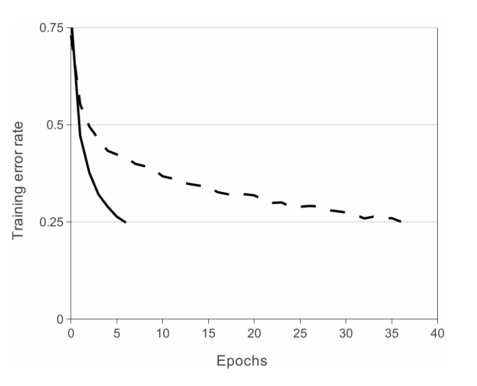
Figure 1: A four-layer convolutional neural network with ReLUs (solid line) reaches a 25% training error rate on CIFAR-10 six times faster than an equivalent network with tanh neurons (dashed line).
그림1: ReLU(실선)가 포함 된 4층 컨볼루션 신경망은 thah 뉴런(점선)이 있는 동등한 네트워크보다 6배 빠른 CIFAR-10에서 25%의 훈련 오류율에 도달합니다.
The learning rates for each network were chosen independently to make training as fast as possible.
각 네트워크에 대한 학습률은 가능한 빨리 훈련을 하기 위해 독립적으로 선택되었습니다.
No regularization of any kind was employed.
어떤 종류의 정규화도 사용되지 않았습니다.
The magnitude of the effect demonstrated here varies with network architecture, but networks with ReLUs consistently learn several times faster than equivalents with saturating neurons.
여기에 설명 된 효과의 규모는 네트워크 아키텍처에 따라 다르지만 ReLU가 있는 네트워크는 포화 뉴런과 등등한 것보다 몇 배 더 빠르게 학습합니다.
3.2 Training on Multiple GPUs
A single GTX 580 GPU has only 3GB of memory, which limits the maximum size of the networks that can be trained on it.
단일 GTX 580 GPU에는 3GB의 메모리만 있으므로 훈련 할 수 있는 네트워크의 최대 크기가 제한됩니다.
It turns out that 1.2 million training examples are enough to train networks which are too big to fit on one GPU.
120만 개의 훈련 예제는 하나의 GPU에 맞지 않을 정도로 큰 네트워크를 훈련시키기에 충분하다는 것이 밝혀졌습니다.
Therefore we spread the net across two GPUs. Current GPUs are particularly well-suited to cross-GPU parallelization, as they are able to read from and write to one another’s memory directly, without going through host machine memory.
따라서 우리는 두 GPU로 늘렸습니다. 현재 GPU는 호스트 컴퓨터 메모리를 거치지 않고 서로의 메모리에서 직접 읽고 쓸 수 있기 때문에 GPU간 별렬 처리에 특히 적합합니다.
The parallelization scheme that we employ essentially puts half of the kernels (or neurons) on each GPU, with one additional trick: the GPUs communicate only in certain layers.
우리가 사용하는 병렬화 체계는 기본적으로 각 GPU에 절반의 커널(또는 뉴런)을 추가하고 하나의 트릭을 추가합니다. GPU는 특정 계층에서만 통신합니다.
This means that, for example, the kernels of layer 3 take input from all kernel maps in layer 2.
이는 예를 들어 계층3의 커널이 겨층 2의 모든 커널맵에서 입력을 받는다는 것을 의미합니다.
However, kernels in layer 4 take input only from those kernel maps in layer 3 which reside on the same GPU.
그러나 계층 4의 커널은 동일한 GPU에 있는 계층 3의 커널 맵에서만 입력을 받습니다.
Choosing the pattern of connectivity is a problem for cross-validation, but this allows us to precisely tune the amount of communication until it is an acceptable fraction of the amount of computation.
연결 패턴을 선택하는 것은 교차 검증의 문제이지만, 이것은 우리가 그것이 계산 양의 허용 가능한 부분이 될 때까지 통신 양을 정밀하게 조정할 수 있게 해줍니다.
The resultant architecture is somewhat similar to that of the “columnar” CNN employed by Ciresanet al. [5], except that our columns are not independent (see Figure 2).
결과 아키텍처는 Ciresan al[5]등이 사용하는 “columnar cnn”과 다소 유사합니다. 열이 독립적이지 않다는 점을 제외합니다.(그림 2 참조)
This scheme reduces our top-1 and top-5 error rates by 1.7% and 1.2%, respectively, as compared with a net with half as many kernels in each convolutional layer trained on one GPU
이 체계는 하나의 GPU에서 훈련 된 각 컨볼루션 계층에 커널이 절반으로 많은 넷과 비교하여 top-1 및 top-5 오류율을 각각 1.7% 및 1.2% 줄입니다.
The two-GPU net takes slightly less time to train than the one-GPU net2.
2-GPU net은 1-GPU net2보다 훈련하는데 약간 더 적은 시간이 걸립니다.
3.3 Local Response Normalization
ReLUs have the desirable property that they do not require input normalization to prevent them from saturating.
ReLU는 포화를 방지하기 위해 입력 정규화가 필요하지 않는 바람직한 속성을 가지고 있습니다.
If at least some training examples produce a positive input to a ReLU, learning will happen in that neuron.
적어도 일부 훈련 예제가 ReLU에 긍정적인 입력을 생성하면 해당 뉴런에서 학습이 발생합니다.
However, we still find that the following local normalization scheme aids generalization.
그러나 우리는 여전히 다음과 같은 지역 정규화 체계가 일반화에 도움이 된다는 것을 발견했습니다.
Denoting by ${a_x}_y^i$ the activity of a neuron computed by applying kernel $i$ at position $(x,y)$ and then applying the ReLU nonlinearity, the response-normalized activity ${b_x}_y^i$ is given by the expression.
위치 $(x,y)$어 커널 $i$를 적용한 다음 ReLU 비선형 성을 적용하여 계산 된 뉴런의 활동을 ${a_x}_y^i$로 표시하면 응답 정규화 된 활동 ${b_x}_y^i$는 다음 식으로 제공됩니다.